| 59.4% |  | United States |
| 8.7% |  | United Kingdom |
| 5% |  | Canada |
| 4.1% |  | Australia |
| 3.5% |  | Philippines |
| 2.6% |  | Netherlands |
| 2.4% |  | India |
| 1.6% |  | Germany |
| 1% |  | France |
| 0.7% |  | Poland |
| Today: | 179 |
| Yesterday: | 251 |
| This Week: | 179 |
| Last Week: | 2221 |
| This Month: | 4767 |
| Last Month: | 6796 |
| Total: | 129366 |
6. The Uses and Implications of the Log-normal Distribution of Drug Use
 |
|  |
| 
| Books - Cannabis and Man |
Drug Abuse
6. The Uses and Implications of the Log-normal Distribution of Drug Use
W. D. M. Paton, Department of Pharmacology, University of Oxford.
A knowledge of the actual rates of drug use is essential for several purposes; for assessing medical or social risk; for considering the reciprocal problems of the effect of social attitudes on use, and of drug use on social attitudes; and for quantitative studies on supply and demand. The information available comes generally from two sources only; seizures, and surveys by questionnaire. For alcohol, purchases and measurements of alcohol blood levels are also sometimes available. For cannabis, there is a particular need to resolve one way or another the apparent conflict between the normal 'stereotype' of use - around 5 mg THC absorbed from an experimental reefer (i.e. c. 0.1 mg/kg a few times), against rates of use up to 100 times this, i.e. 10 mg/kg daily or higher, recorded in the WHO Report (No. 478: 1971). The medical and social picture would, of course, be quite different as between a
uniform rate of use through a population, and a generally abstinent population with a small group of heavy users.
Ledermann (1958) introduced into alcohol studies the log-normal distribution; Lindt and Schmidt (1968) followed this up for alcohol, and Smart and his colleagues (1970) for general use. If one collates the available
data from these and other sources, there are signs that a coherent picture of some heuristic use emerges. Since Ledermann's treatment is somewhat cryptic, and includes the assumption of a correlation between the mean and the standard deviation of the distribution, I have used a simpler and more empirical approach, the use of logarithmic probability paper - a procedure very familiar to pharmacologists since the introduction of this mode
of analysis by Gaddum in 1933. It is required only that the data are such that rates of use can be assigned to the whole population, without deficit or overlap. The procedure is applied to cumulated data rather than to frequency distribution. When plotted, as % using a drug at a given rate or higher, the probability ordinate scales percentages in such a way that if the distribution is normal, a straight line is produced, whose intercept at 50 per cent gives the median and whose slope gives the standard deviation. Thus, taking Binnie's data on cannabis use (1969), recalculating to include non-user students, we have:
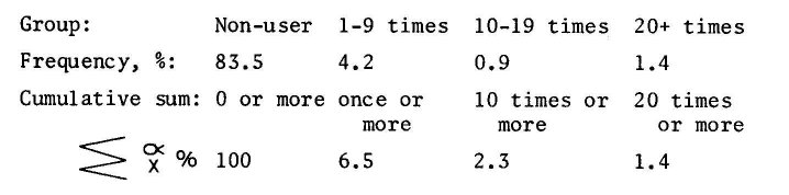
Cumulation here is 'from the right', since for the moment it is the proportion taking a given dose or more that is important.
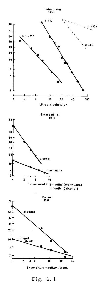
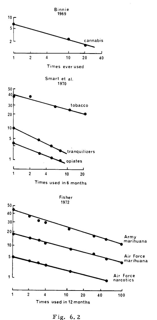
Figures 6.1 and 6.2 show these data plotted. They also include data from Smart and his colleagues (Canadian schoolchildren), from Ledermann (French adults), and from Fisher's study (1972) in the USA Armed Services. First,
all the data fit a log-normal distribution well. Second, there appear to be two patterns: one for alcohol, with a lower standard deviation (of the order of 2-5 x in geometrical terms); the other for cannabis, and in fact
it seems for most other drug use reported, including other illicit drugs, tranquillizers, and smoking, with a standard deviation of the order of 50 x or higher. The relative constancy of the standard deviations is remarkable, considering the wide range of populations involved, and of ages, rates of use, and drugs.
Graphs of the percentage of various populations using certain drugs at a given rate or higher, plotted with probability scale for percentage ordinate, and logarithm of rate of use for abscissa. Data from Ledermann (1956), Binnie (1969), Smart et al. (1970) and Fisher (1972).
IMPLICATIONS
1. It appears to be worth while to analyse the data in this way, and to make sure that data are obtained in suitable form - some data are not so obtained. At the least, one is then able to express the results of a survey conveniently by means of two quantities, the median rate of use or the mean rate of use, and the standard deviation. Consistency or inconsistency of behaviour, not otherwise easily apparent, can then be recognized.
2. It has been suggested that the fact of a lognormal fit throws light on causes. In general, I think this is not the case. Any variable phenomenon which is the outcome of a large number of small variables tends rapidly to normality, as was shown by Gauss, Laplace and Bessel; and the logarithmic transformation simply implies that it is proportionate rather than absolute variations that are relevant, as is normally the case in drug action. An extra sherry a day to someone only taking a glass a day is a substantial increase in alcohol intake; to a bottle-a-day man, it is trivial, while another bottle a day would be significant. The log-normal fit could mean only that we are dealing with a multifactorial aspect of drug action. It does imply, probably, that there are not two contrasted sub-populations; it does not imply, however, that there may not be as few as 4 or 5 sub-populations, since the sum of several normal curves is liable to be very hard to distinguish from a single one.
3. The most important aspect seems to me that of the magnitude of the standard deviation - i.e. of the steepness or flatness of the lines. To take an example, suppose we have a drug which 10 per cent of the population take once a month or more times a month, and a minute fraction 100 times or more a month. But for a standard deviation of 50 x (like tobacco, cannabis and others), 3 per cent will take it 10 or more times a month and only a little under 1 per cent will take it 100 times or more a month. With high standard deviations, the proportionate incidence of high rates of use increases greatly. This seems to me a very important fact about drug use; and, for cannabis, it implies that the WHO collation is, in fact, completely correct. For such a drug, in addition, pharmacological exploration of the effect of high doses becomes essential.
4. As a final aspect, which can not be developed, one may note that one can begin to approach a calculation of total amounts consumed, to construct Lorenz-type curves, to relate patterns of use with estimates of supply, and to make some estimate, given an estimated mean rate of consumption, of the numbers of people using drug at a given rate or higher. In short, there are reasons for hoping that it is possible to do for other drugs what Ledermann did for alcohol.
REFERENCES
Binnie, H.L. (1969). The attitude to drugs and drug-takers of students at the University and Colleges of Higher Education in an English Midland city. Vaughan Paper No. 4, Dept. of Adult Education, The University, Leicester.
Fisher, A.H. (1972). Preliminary findings from the 1971 Department of Defence survey of drug use. Human Resources Research Organization Technical Report 72-8.
Gaddum, J.H. (1933). MRC Reports on Biological Standards III. Methods of Biological Assay Depending on a Quantal Response. Special Report Series No. 183. H.M.S.O.
Ledermann, S. (1956). Alcool, Alcoolisme, Alcoolisation; Données Scientifiques de Caractère Physiologique, Economique et Social. Institut National d'Etudes Démographique, Travaux et Documents, Cahier No. 29, Presses Universitaires de France.
de Lindt, J. and Schmidt, W. (1968). The distribution of alcohol consumption in Ontario. Q.J. Stud. Alc. 29, 968-973.
Smart, R.G., Fejer, D. and Alexander, E. (1970). Drug use among high school students and their parents in Lincoln and Welland Counties. Addiction Research Foundation, Toronto, Canada.
WHO Technical Report Series No. 478 (1971). The Use of Cannabis. World Health Organization, Geneva.
DISCUSSION
DEFINITIONS OF 'HEAVY USE'
Referring to Professor Paton's offer of a partial definition of heavy use as 'that point when accumulation in the body occurs', Dr Cameron pointed out that many heavily-used drugs, such as cocaine, accumulated very little, yet were often used frequently. Professor Paton stressed that accumulation was only one aspect of heavy use, and that pharmacologists could not predict or define the meaning of 'heavy use' apart from accumulation, without considering somatic effects.
Dr Edwards pointed out that although the alcohol intake per year of two populations might be similar, different populations may often have different distributions of use through time. One can drink a little regularly, or a lot, more seldom. 'This is of more than theoretical importance: it may very much influence the social impact of the drug, and may quite require different social policies'.
IS THE GRAPH AFFECTED BY PROPERTIES OF THE DRUG?
Professor Paton suggested that there is a consistency of distribution of frequency of use 'which I think is telling us something not about drugs, but about patterns of human behaviour of this kind'.
Mr Hasleton asked if there was an implication that one could validly extrapolate the curve to describe patterns of very low and very high use, and Professor Paton said that he would be reluctant to extrapolate without empirical basis. Ledermann had made the assumption that one can't take more than a certain amount of any drug, therefore there has to be a right-hand limit to the curve. Once you say that you are putting a constraint on the rest of the curve.
Mr Hasleton and Dr Edwards asked whether the properties of the drug influenced the distribution of frequency of use. Dr Edwards suggested that the shape of the curve was partially determined by the population, partially by the culture, its economies and mores, and partly by the drug. 'Supposing we have drug X, which is non-dependence producing, and that we know its distribution of frequency of use curve. Let us now introduce into drug X a dependence producing potential. Will this change in the characteristic of the drug in no way alter the shape of the curve?' Professor Paton suggested that one could work towards an answer by obtaining distribution curves for commonly used, freely available more 'neutral' drugs, such as nasal drops, aspirin etc.
IMPLICATIONS FOR MINIMISATION OF HEAVIER USE
Dr Miles congratulated Professor Paton on his paper, and added, 'I've been advocating for a long time micro-economy studies , where the price of various drugs is varied for a captive audiance. The obvious ones to vary, of course, are alcohol and marijuana. It would be very interesting to see, when people are in a productive situation, when they have access to drugs that they have to pay for, how you could change the curves presented by Professor Paton'.
Professor Paton replied that: 'If you wish to diminish the amount of heavier use, there are two ways to do it. You can either reduce the total consumption down or you can try to find a way to move only the heavier users.'
Dr Cameron agreed saying that one should stress that there were two possible ways to reduce heavier use. 'First, you can change the mean, or the mode: that is to change the pattern of drinking of the whole population, to shift
the whole curve downward. Or you may have another programme which is aimed at changing the standard deviation, aimed primarily at the heavier user and not at the whole population. It needs to be stressed that one need not approach one or the other programme exclusively.'
Professor Paton pointed out that it might not be necessary to talk of heavy users as a separate class. A system might be evolved which applies increasing pressure as use goes up.
Dr Smart said that there were few well studied situations where drug use was going down 'so one really can't be sure whether it's possible to change the standard deviation or mean or both.'
| < Prev | Next > |
|---|